How to read a stat-arb backtest without fooling yourself

A backtest is a story. The interesting question is which version of the truth it is telling.

Every stat-arb platform shows a backtest in its marketing material. Almost all of them have at least one of five problems that turn the equity curve into fiction. Knowing the problems lets you read any backtest like a person reading a financial statement: the numbers matter less than which methodology produced them.

What follows is a short field guide. The references at the bottom point you at the academic literature on each item. The full technical treatment with formulas is in the implementation paper.

A backtest with tunable parameters (entry threshold, exit threshold, lookback window, hedge-ratio refit cadence) needs to tune those parameters on data the evaluation does not see. Otherwise it is reporting how well the parameters fit the history. That is not the question.

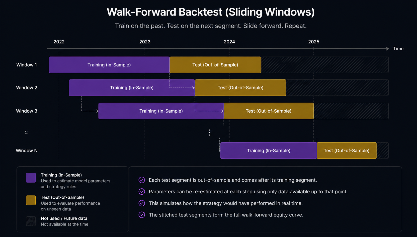
The standard fix is walk-forward partitioning (Bailey, Borwein, Lopez de Prado and Zhu 2014). Split the data into rolling training windows and sequential test windows. Tune on training, evaluate on the immediately following test, slide forward, repeat. The aggregated test-window PnL is the walk-forward out-of-sample backtest. That is the equity curve you should be looking at, not the in-sample-best version.

If a backtest report does not specify walk-forward windows and step sizes, assume the parameters were fit on the same data as the evaluation.

The historical price path that actually happened is one draw from the distribution of paths that could have happened. The fact that your strategy worked on the realised path is weak evidence that it works on the path that follows.

Lopez de Prado (2018) is unsparing on this point. Robust validation requires resampling. The two standard approaches:

A defensible backtest shows you both the realised equity curve and the resampled distribution. The width of the distribution tells you the actual uncertainty around the point estimate.

Three formal tools developed by Bailey and Lopez de Prado quantify how seriously to take a reported Sharpe ratio.

Probabilistic Sharpe Ratio (PSR). The probability that the true Sharpe exceeds a threshold, given the observed Sharpe and the higher moments of the return distribution. Adjusts the standard error of the Sharpe estimator for non-normality (Bailey and Lopez de Prado 2012). If a strategy reports a Sharpe of 1.5 but the PSR against the benchmark of 1.0 is only 60%, the reported Sharpe is less impressive than it looks.

Deflated Sharpe Ratio (DSR). Extends PSR for the case where the reported strategy is the best of N tested strategies. Adjusts the threshold downward by the expected maximum of N independent Sharpe ratios under the null. If the DSR is below 0.5, the reported Sharpe is consistent with selection-bias noise (Bailey and Lopez de Prado 2014).

Probability of Backtest Overfitting (PBO). The probability that the in-sample best strategy is below the median out of sample. Computed via combinatorial cross-validation (Bailey, Borwein, Lopez de Prado and Zhu 2017). PBO of 1.0 means the selection process has no out-of-sample skill.

These three metrics are diagnostic, not gating. A strategy selected purely by maximising in-sample Sharpe with PBO close to 1 should be discarded. A strategy with DSR above 0.95 and PBO close to 0 has stronger statistical support than its raw Sharpe alone suggests.

Pairs trading is high-turnover. A backtest that assumes mid-price fills and zero transaction cost overstates achievable PnL by an amount that often exceeds the gross edge.

A defensible cost model includes:

• Bid-ask spread. Fills occur at the side of the book, not the midpoint.
• Slippage. For order sizes that exceed top-of-book, the effective fill walks the book. Almgren et al. (2005) is the standard reference for the empirical scaling laws.
• Exchange fees at the user s tier, including the maker rebate vs taker charge distinction.
• Funding payments for perpetual futures at the venue cadence (typically eight-hourly).
• Borrow costs for the short leg in equity markets.
• Latency between signal generation and exchange acknowledgement.

If a stat-arb backtest reports a high Sharpe and does not name its fee, funding and slippage assumptions, the high Sharpe is probably not surviving the cost model it has not built.

A pair universe built from currently-tradeable assets excludes assets that were delisted, merged or otherwise removed from the historical record. The resulting backtest overstates pair stability because the failures have been silently removed.

The fix is point-in-time universes: at each historical time t, restrict the backtestable universe to assets that were listed, tradeable and met the strategy s liquidity criteria as of t. Constructing point-in-time universes requires complete historical listing and delisting metadata.

A related concern: the pairs evaluated must themselves be selected using only information available at the formation time. A backtest that uses 2024 cointegration tests to pick pairs and then trades those pairs over 2018 to 2023 is selecting on the future. The right pair set differs at each historical time.

A defensible pairs-trading backtest report includes, at minimum:

1. Universe description with point-in-time membership criteria.
2. Method description sufficient to reproduce: pair selection, hedge-ratio estimator, trading rule, position sizing, exit conditions, transaction-cost model.
3. Walk-forward partitioning specification: window lengths, step size, parameter optimisation procedure per window.
4. Aggregate performance: out-of-sample PnL, annualised Sharpe (and PSR / DSR), maximum drawdown, win rate per trade, turnover, transaction cost as fraction of gross PnL.
5. Robustness diagnostics: block-bootstrap or Monte Carlo PnL distribution; PBO if a parameter grid was searched; sensitivity to principal parameter choices.
6. Cost decomposition: PnL with and without each transaction-cost component.

Reports that omit walk-forward partitioning, show a single equity curve without a resampled distribution, or do not disclose the transaction-cost model are not interpretable as evidence of deployable performance. The Hedgicore methodology paper documents the backtest scope in §5. The full technical treatment is at Pairs Trading Implementation §4.

References

- Bailey, D.H. and Lopez de Prado, M. (2012). The Sharpe ratio efficient frontier. Journal of Risk 15(2).
- Bailey, D.H. and Lopez de Prado, M. (2014). The deflated Sharpe ratio. Correcting for selection bias, backtest overfitting and non-normality. Journal of Portfolio Management 40(5).
- Bailey, D.H., Borwein, J.M., Lopez de Prado, M. and Zhu, Q.J. (2014). Pseudo-mathematics and financial charlatanism. The effects of backtest overfitting on out-of-sample performance. Notices of the American Mathematical Society 61(5).
- Bailey, D.H., Borwein, J.M., Lopez de Prado, M. and Zhu, Q.J. (2017). The probability of backtest overfitting. Journal of Computational Finance 20(4).
- Künsch, H.R. (1989). The jackknife and the bootstrap for general stationary observations. Annals of Statistics 17(3).
- Politis, D.N. and Romano, J.P. (1994). The stationary bootstrap. Journal of the American Statistical Association 89(428).
- Lopez de Prado, M. (2018). Advances in Financial Machine Learning. Wiley.
- Almgren, R., Thum, C., Hauptmann, E. and Li, H. (2005). Equity market impact. Risk 18(7).
- Bonton AI, Hedgicore Research (2026). Pairs Trading Implementation. Hedge Ratio Estimation, Trading Rules and Backtesting. v1.0.
Hedgicore is a real-time pairs analytics platform powered by the Hedgicore Engine. Built by the team at Bonton AI.
Risk disclaimer: Hedgicore is an analytics platform. It does not execute trades or provide financial advice. All trading carries risk of loss.